What is Sigma Quality Level?

View All Blogs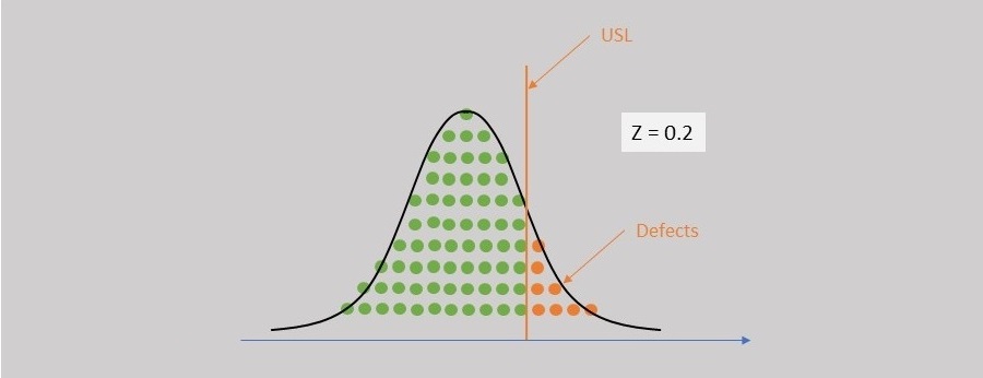

Sigma Quality Level is a number that provides a quantitative measure of the capability of any process. It is usually indicated by the letter Z or SQL. It can be used to describe if the process is capable of meeting customer requirements. Hence, in order to calculate the Sigma Quality Level, we need two pieces of information: customer requirements and process performance data. In this module, we will look at how to compute the Sigma Quality Level for different situations and also discuss some of the limitations of the Sigma Quality Level metric.

A. Calculating Sigma Level for Normally Distributed Continuous Data

If your data type is continuous and is normally distributed with a single specification limit (let’s say without loss of generality the Upper Specification Limit USL), then the Sigma Level indicates the number of standard deviations (s) that you can fit between the process average (xbar) and the customer defined specification limit. This can be expressed mathematically as follows:

For example, if we are interested in the capability of the temperature of the room and the temperature of the room averages around 20 degrees with a standard deviation of 1.5 degree and the customer specification limit is 23 degrees, then using the above formula the Sigma Level would be 2 (or it is a 2 Sigma process).

A very capable process will have a large Sigma Level while an incapable process will have a small Sigma Level. A large value for the Sigma Level indicates that the process is operating far away from the customer specification limits and hence there is less chance of making defects. The best possible process in the world would have a Sigma Level of +∞ (infinity) and the worst possible process in the world would have a Sigma Level of –∞ (negative infinity). A process with 50% defects (DPMO = 500,000) would have a Sigma Level of 0. Usually, a process with a Sigma Level of 6 or greater is usually considered as an excellent process.

Calculating Sigma Level from DPMO

If you know the capability of a process as DPMO number (see previous article on DPMO), then you can compute an equivalent value of Sigma level using the following approach. Divide the DPMO by 1,000,000 to get the area under the curve. The area under the curve is an indication of probability of defects. Use a unit-normal distribution (with mean = 0, and standard deviation = 1) and calculate the Sigma Level that corresponds to this distribution that provides the same defect area to the right. This approach is shown in the following figure.
For example, if the DPMO = 45000, then Area = 0.045000 and hence Z = 1.7. Note that this sigma level does not assume a 1.5 Sigma shift that is covered later in this article.

If you have a bilateral specification, where both the USL and LSL are specified, then the Sigma Level is calculated by first calculating the total DPMO on both sides of the specification limits as follows:

This DPMO value can be translated to the Sigma Level using the methodology described in Section A. This Sigma Level is also called ZBench.

Even though by the strict definition, the Sigma Level only applies for a continuous data that is normally distributed, we can calculate an equivalent Sigma Level for other types of distributions for continuous data sets or even for discrete data sets. In the following sections, we will deal with how to calculate the Sigma Level for different types of data.

B. Sigma Level for a Non-normal Continuous Distribution

If the data is not normally distributed, we cannot use the formulae described earlier to calculate the Sigma Level. There are two approaches you can use to calculate the Sigma Level for non-normal distributions. In the first approach, you can transform the non-normal data to a normal distribution and then calculate the Sigma Level using the methods described above. You could use either the Box-Cox transformation or the Johnson transformation to transform the data to a normal distribution. One thing to note is that in addition to the data the specification limits should also be transformed before you calculate the Sigma Level. The following figure shows non-normal data that has been transformed using the Box-Cox transformation. The resulting Sigma Level is 1.55.

In the second approach, you can fit a non-normal distribution to the data (such as a Log-normal distribution, Exponential distribution etc) to the data. Once you have a distribution fit to the data, you can calculate the area under this curve that lie outside the specification limits. This area can be used to estimate the DPMO. Once we have the DPMO number, you can use the methodology described in section A to calculate the Sigma Level. The following figure shows a curve fit (Beta distribution) that is fit to the non-normal data. The resulting Sigma Level is 1.54.

So, which method should you use? If you know for a fact that based on the physical properties of the data that the data follows a specific distribution, then you can use the curve-fit method to fit that distribution to the data. However, if you have no a-priori knowledge of the distribution, then the transformation method can be used. Box-Cox transformation should be tried first as it is relatively easy to understand and explain. However, Box-Cox transformation may not always be successful in transforming the data to a normal distribution. In Box-Cox is not successful, then you could try to transform the data using the Johnson transformation.

C. Sigma Level for Discrete Distribution

For discrete data, we can also estimate the Sigma Level by first calculating the DPMO and then using the methodology described in section A to calculate the Sigma Level. For example, if the number of defects = 10, number of units = 100 and the Opportunities for error per unit = 5, then DPMO can be calculated as:

This DPMO translates to a Sigma level of Z = 2.054.

Short Term and Long Term Sigma Level

When you calculate the Sigma Level, you sometimes need to distinguish between Short-Term and Long-Term. Short-Term data is data that is collected for a short period of time when typically only common causes are present. Long-Term data is data that is collected for a long period of time when both common and special causes are present. If Short-Term data is used to calculate the Sigma Level then we can denote the Sigma Level as ZST and for Long-Term Sigma Level as ZLT.

In literature, you will find that some people translate between the Short-Term and Long-Term Sigma Level using a 1.5 Sigma Shift assumption. This relationship is usually expressed as: ZST = ZLT + 1.5

The 1.5 number is “pulled” out of thin air without strong statistical foundation. Hence, we recommend that you not use this shift in your calculations. In addition, it is also not clear what period of time can be considered Long-Term. For example, both six months and one year can be considered long term! Not all processes would deteriorate by a Sigma Level of 1.5 (even assuming that on average it drop by 1.5). Instead, we recommend that you calculate the Sigma Level based on the data you have and clarify if your Sigma Level is calculated using Short-Term data or Long-Term data without using the 1.5 shift assumption.

Limitations of Sigma Level

There are several limitations to use of Sigma Level for quantifying the capability of a process. Some of the common problems or issues with use of Sigma Level is listed below:

• Sigma Level is a non-linear metric. For example, to go from Z =1 to Z = 2 would require an improvement from 85% to 97.5% while to go from Z = 2 to Z = 3 would require an improvement from 97.5% to 99.86%.
• Since some people use the 1.5 Sigma Shift while others don’t, it is not clear what the “true” value of the Sigma Level is.
• People may use the wrong approach to calculate the Sigma Level which may result in incorrect values and/or interpretation.
• A good value of Sigma Level depends on the process. For example, a person might interpret Z = 6 as a good process but the process performance may not be acceptable – for example aircraft landings require Z = 8 or above.

---

Follow us on LinkedIn to get the latest posts & updates.